Training models
Consider a basic linear regression model there are two ways train it :
A.Direct “Closed form”
The equation directly computes the model parameters that best fit the model to training set (that is, the model parameters minimize the cost function over the training set )
B.Iterative Optimization approach
This is called gradient descent (GD) that gradually tweaks the model parameters to minimize the cost function over the training set which eventually converges to the same set of parameters that is obtained in the first method
Linear Regression
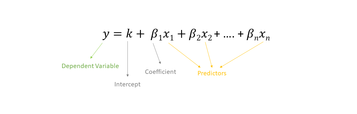
Equation of a linear regression model is :
 The most common error measure used to evaluate such models is Root Mean Square Error (RSME). Hence we choose a model that reduces the cost function. However in practice it is easier to reduce the MSE (Mean Square Error) rather than RMSE. The MSE cost function is given by

Gradient Descent
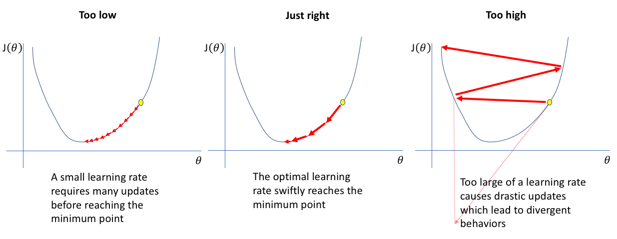
This is a general optimization algorithm used to find solutions for a wide range of problems. The general idea of gradient descent is to gradually tweak parameters in order to minimize the cost function. An important parameter of gradient descent is the size of steps which is determined but the learning rate hyperparameter. If the learning rate is very small the algorithm will have to run through many iterations in order to converge to a solution. On the other hand if the learning rate is too high, the algorithm might tend to diverge from the actual minimum value
 Not all the cost functions have a bowl like shape, they may have ridges,plateaus,etc. This leads to drawbacks of gradient descent. Sometimes the value it converges to might be the local minima and not the global minimum, which may be the actual minimum value. However, when you consider the MSE cost function, the function is convex, hence there is no local minima but just a global minima.
While using GD ( Gradient Descent) make sure to scale the values using
Not all the cost functions have a bowl like shape, they may have ridges,plateaus,etc. This leads to drawbacks of gradient descent. Sometimes the value it converges to might be the local minima and not the global minimum, which may be the actual minimum value. However, when you consider the MSE cost function, the function is convex, hence there is no local minima but just a global minima.
While using GD ( Gradient Descent) make sure to scale the values using StandardScaler so that it converges faster
Batch Gradient Descent
In Batch Gradient Descent, all the training data is taken into consideration to take a single step. We take the average of the gradients of all the training examples and then use that mean gradient to update our parameters. Batch Gradient Descent is great for convex or relatively smooth error manifolds. In this case, we move somewhat directly towards an optimum solution.
Stochastic Gradient Descent
The main problem with batch gradient descent is that it uses the whole training set to calculate the gradient at every step, making it very slow. However stochastic gradient descent just picks a random instance as the training set at every step and computes the gradient based on that descent. This makes the algorithm much faster and makes it possible to train huge datasets. Due to its stochastic nature, this algorithm is much less regular than Batch Gradient Descent. Instead of gradually decreasing until it reaches the minimum, the cost function will bounce up and down decreasing on average. As the algorithm bounces all over the place and finally settles down. So, once the algorithm stops the final parameter values are good, but are not optimum. When the cost function is very irregular with great jumps, hence it may jump out of the local minima, giving it a greater chance to find the global minima
Mini-Batch Gradient Descent
This is more of a combination of both SGD (Stochastic Gradient Descent) and GD (Batch Gradient Descent). Mini GDs calculate the gradients over random sets of instances called mini-batches. The main advantage of Mini-Batch GD is that you can get a performance boost from hardware optimization of matrix operations, especially using GPU’s. The algorithm is less erratic when compared to SGD, making it also harder to escape from the local minima.
Polynomial Regression
If the data is more complex than a simple straight line, you can use a linear model to fit non-linear data. This is done by adding powers to each of the features as new features. This is called polynomial regression.
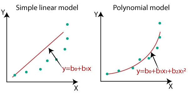 At times if you polynomial regression, you are more likely to fit better than a plane linear regression.
Bias-Variance Tradeoff
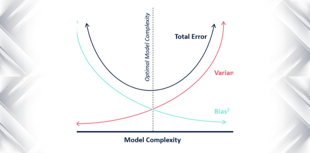
A models generalization error can be a combination of 3 different errors :
A. Bias
This part of the generalization error is caused due to the wrong assumptions.This involves assuming the data is linear, when it may be actually quadratic. High-bias models are most likely to underfit the data
B. Variance
This is due to the model’s excessive sensitivity to small changes in the training data. High degree models tend to give high variations and this ultimately leads to overfitting of the data
C. Irreducible Error
This is caused due to the nosiness in the data. Only way to reduce this error is to clean up the data.
The tradeoff is between Bias and Variance. If Variance is high then the bias is small. However if the bias is high, then the variance is small.
Regularized Linear Model
A good way to reduce overfitting of data on the model is to regularize the model. This can be done by reducing the degree of freedom. For Linear model’s regularization is achieved by constraining the weights of the model
Ridge Regression
It is a regularized version of linear regression. 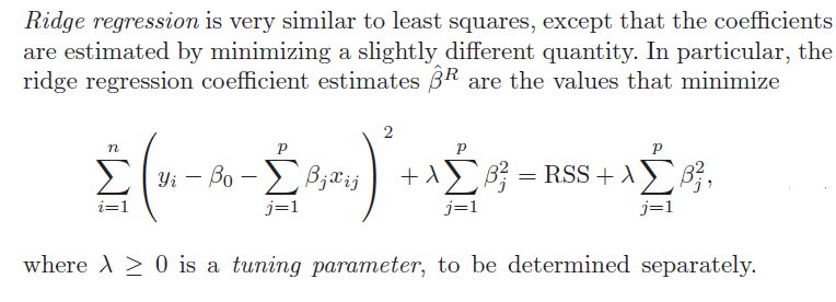 The regularization term forces the learning algorithm to not fit the data but also keeps the model’s weights as small as possible. It is important to note that the regularization should be added to cost function only while training. To evaluate the model’s performance, we would use the unregularized performance measure. The hyperparameter “lambda” controls how much you want to regularize the model. If lambda=0, we get a simple linear model. If the lambda is very large, we ultimately get almost all weights as 0, resulting in a flat line through the data’s mean.
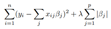
Lasso Regression
This is a modification of the ridge regression. This uses a L1 norm instead of L2. The equation is given by
Elastic Net
This is a combination of both lasso and ridge regression. The equation is given by :
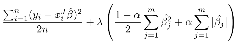 The regularization term is controlled by a term alpha. When alpha=0 we get a purely Ridge regression and when alpha=1, then it is purely Lasso regression.
For basic regression it is always suggested to use some kind of regularization. Usually the order of regularization tried is
The regularization term is controlled by a term alpha. When alpha=0 we get a purely Ridge regression and when alpha=1, then it is purely Lasso regression.
For basic regression it is always suggested to use some kind of regularization. Usually the order of regularization tried is
Ridge Regression ->Elastic Net ->Lasso Regression

Early stopping
This is simple technique in which we stop iterating once the minimum is reached.There are three elements to using early stopping; they are:
- Monitoring model performance.
- Trigger to stop training.
- The choice of model to use.
Logistic Regression
Just like a linear regression model, a logistic regression model computes the weighted sum of the input features. However instead of outputting the result directly like linear regression, It outputs the logistic of the result. The logistic used is a sigmoid function and the output is between the numbers 0 and 1. The equation of sigmoid is given by

Once the logistic model has estimated the probability it can classify an instance.
The cost function
The cost function in logistic regression is given by
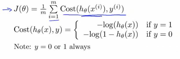
The cost function over a training set is simply the average cost over all training instances. It is expressed as an expression called log loss. Logistic regression models can be regularized using L1 and L2 penalties. For logistic regression the regularization parameter is the inverse of that of “lambda”. Higher the value,the less the model is regularized.
Softmax Regression
Softmax Regression (synonyms: Multinomial Logistic, Maximum Entropy Classifier, or just Multi-class Logistic Regression) is a generalization of logistic regression that we can use for multi-class classification (under the assumption that the classes are mutually exclusive). In contrast, we use the (standard) Logistic Regression model in binary classification tasks. The idea is simple: when given an instance ‘x’, the softmax regression model computes a score Sk(x) for each class ‘k’. Then the softmax function is applied to find the probability of each class.
The softmax function which computes the exponential of each score and then normalises them.