Support Vector Machines
Support Vector Machines (SVMs) is a powerful and versatile model capable of linear and non-linear classification, regression and even outlier detection.
The basics of Support Vector Machines and how it works are best understood with a simple example. Let’s imagine we have two tags: red and blue, and our data has two x and y. We want a classifier that, given a pair of (x,y) coordinates, outputs if it’s either red or blue. We plot our already labeled training data on a plane. A support vector machine takes these data points and outputs the hyperplane (which in two dimensions it’s simply a line) that best separates the tags. This line is the decision boundary: anything that falls to one side of it we will classify as blue, and anything that falls to the other as red.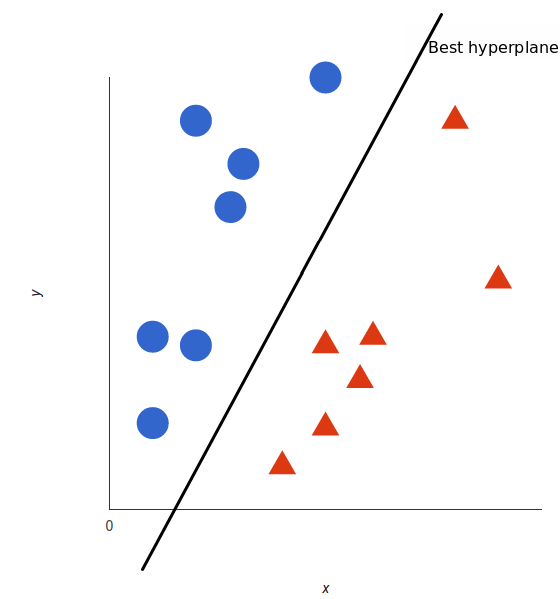
Linear SVM Classification
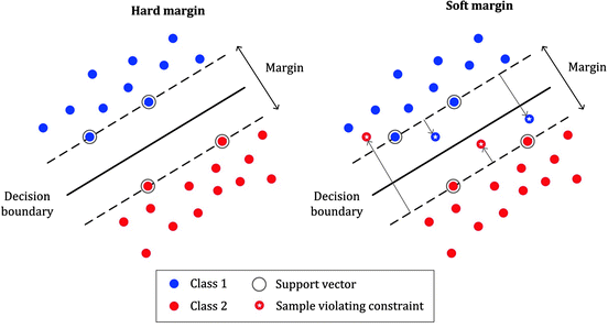
The hyperparameter ‘c’ in SVM is used to specify the type of SVM. It can be of two: A. Hard Margin: There should be no outliers on the street. B. Soft Margin: There can exist outliers on the chosen street. If the value of c is smaller it would lead to wider streets and more margin violations.
Unlike logistic regression classifiers, SVM’s do not use probabilities. You can use the SGDClassifier that uses Stochastic Gradient Descent to train a linear SVM classifier. This does not converge as fast as linear SVC, but can be used for large datasets
Non linear SVM Classification
Sometimes the dataset would be non-linear. The best way to represent that kind of data is to add more features such as polynomial features.
Polynomial Kernel
Adding polynomial features can work with all types of machine learning algorithms. If the degree is higher it can be slow, however a low degree can not be used to handle complex datasets properly. However with SVM you can use a ‘kernel trick’. This makes it possible to get results as if you added a polynomial feature of high degree without even actually doing so.
Adding similarity features
Another technique to tackle nonlinear problems is to add features computed using a similarity function that measure how much an instance resembles a particular landmark.
Gaussian RBF
Just like polynomial feature method, the similarity features method is useful for any ML algorithm, The RBF kernel has two hyperparameters- ‘gamma’ and ‘c’. C is the regularization parameter. It is inversely proportional to alpha. Lower the value of C the more the model is regularized. Increasing the value of gamma makes the bell shaped curve narrower and as a result each instance’s range of influence becomes smaller. This means that ‘gamma’ is also a regularization parameter. If your data is overfitting, it would be wise to reduce it.
SVM Regression
The SVM algorithm is versatile and can be used for regression as well. The trick is to inverse the objective, that is instead of finding the largest possible street between two classes while limiting the margin. For regression we try to fit as many instances on the street while limiting the margin restrictions
Decision Functions and Predictions
The linear SVM classifier model predicts the class of a new instance by simply computing the decision function. If the result is positive, the predictive class is the positive class or else negative class