Ensemble Learning and Random Forests
If you ask a complicated question to thousands of random people. It is said that the aggregate answer is better than the answer given by experts. This is called wisdom of the crowd. Similarly if you aggregate the predictions of a group of predictors, you will often get a better prediction than the best individual predictor. A group of predictors is called an ensemble and hence this technique of using many predictors is called Ensemble Learning. For instance you can train a group of decision trees classifiers and each on a different random subset of the training set. To make predictions, you need to obtain the predictions of all the individual predictors and then predict the class that gets the most votes. Such as ensemble of decision trees is called Random Forests.
Voting Classifiers
Suppose you have trained a few classifiers,each having about 80% accuracy. Let’s say you may have Logistic Regression, SVM, K-nearest Classifier, Random forests, etc. A very simple classifier is to aggregate the predictions of each classifier and predict the class that gets the most votes. It is seen that very often, such a kind of voting classifier achieves a score higher than the best classifier in the ensemble. This possible because it is based of the wisdom of the crowd notion. The version of the law used in machine learning states that if you build an ensemble containing 1000 classifiers that are individually correct only 51% of the time (close to random predictions). You can hope to achieve an accuracy of 75% from the ensemble. However this is only possible if the models are independent and make uncorrelated errors. This is not the case as they are trained using the same training set most of the time. This reduces the ensemble accuracy to some extent.
Bagging and Pasting
One way to obtain a diverse classifier is to use different algorithms. Another approach is to use the same training algorithm for every predictor but to train them on different random subsets of the training set. When the sampling is performed with replacement it is called Bagging, otherwise the sampling is performed without replacement and is called Pasting. Basically both bagging and pasting allows the training instances to be sampled several times for the same predictor. Once all the predictors are trained, an ensemble can make a prediction for a new instance by simply aggregating the predictions of all predictors.
Note the aggregating function is often just a simple statistical mode for classification or a the statistical average for regression
Each individual predictor has a higher bias than if it was trained individually on the original training set. However, aggregation reduces both bias and variance. One of the reasons bagging and pasting is so popular is that they scale very well. For instance, you can train predictors in parallel via different cores or servers
Random Patches and Random Subspaces
The bagging classifier also supports sampling features as well. This sampling is controlled by the hyperparameters max_features and bootstrap_features in sklearn. They are particularly useful when you are dealing with high - dimensionality inputs such as images. Sampling both training instances and features is called Random Patches Method. While sampling only the features is called Random Subspaces Method.
Random Forests
It is an ensemble of decision trees, generally trained by the bagging method with the max_samples set to the training set. Instead of building a BaggingClassifier with DecisionTreeClassifier you could call the RandomForestClassifier that is found in sklearn. This is more optimized and convenient. With a few exceptions RandomForestClassifier has all the hyperparameters that a DecisionTreeClassifier and BaggingClassifier has. This classifier also introduces extra randomness when growing trees. So, instead of searching for a very feature to split a node, it searches for the best feature among a random subset of features. This results in a much more diverse tree, again trading high bias for a lower variance.
Extra Trees
While growing a tree in Random forests, at each node only a random subset of the features is considered. The question arises if it is possible to make the trees even more random by also using random thresholds for each feature, rather than searching for the best possible threshold. A forest of such extremely random trees is called an extremely Randomized Trees Ensemble. This again trades high bias for lower variance. This also makes extra trees faster than the regular random forests.
Another great quality of random Forests is that it helps to measure the relative importance of features
Boosting
Boosting was originally hypothesis boosting and refers to the ensemble learning method in which several weak learners are combined to form a strong learner. The general idea of boosting is to train its predictors sequentially improving on its predecessor. There are many boosting methods such as :
A. AdaBoost
One way for its predictor to correct its predecessor is to pay a bit more attention to the training instances that the predecessor underfitted. This results in the new predictor to focus more and more into the hard cases. This technique is called AdaBoost. For example, to build an AdaBoost classifier based on the first base classifier ( such as decision trees), the first base classifier is trained on the training set. The relative weight of the misclassified training instances is then increased. A second classifier is trained using the updated weights. It makes predictions and the weights are again updated. This cycle goes on.
If AdaBoost is overfitting you can control it by reducing the number of estimators.

B. Gradient Boosting
Just like AdaBoost, gradient boosting works sequentially adding predictors to an ensemble, each one correcting the predecessor. The difference is instead of tweaking the weights at every iteration like in AdaBoost, this method tries to fit a new predictor to the residual errors made by the previous predictors. A simple example can be shown using decision trees. This is called gradient boosting decision trees. The learning rate hyperparameter scales the contribution by each tree. If you set the learning rate below 0.1 it needs more trees in the ensemble to fit the training set, however this would generalize better. This method is called shrinkage.
Sometimes increasing the number of estimators and reducing the learning rate can also lead to the overfitting of data. This can be controlled by early stopping using the stage_predict method that returns an iterator of the predictions made by the ensemble at each stage of training. You can also use early stopping by keeping the hyperparameter warm_state=True. This keeps the tree as it is with incremental training.
The GRBT class in sklearn also has a hyperparameter subspace which specifies the fraction of the training instances that could be used to train the tree, This however trades higher bias for a lower variance.
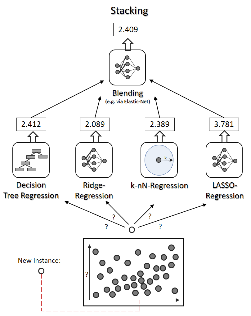
Stacking
This is based on the simple idea that instead of using a function to aggregate the predictors in the ensemble , why don’t we train a model to do this. The final model aggregates the predictors in a so-called blender.