Unsupervised Learning Algorithms

26 May 2021 - 5 mins read time
Tags: Hands-On Machine Learning2

Although most applications of ML are based on supervised learning, most of the data available in the real world is unlabeled . The most important unsupervised learning algorithms fall into 3 main categories :

• Clustering
• Anomaly Detection
• Density Estimation

Clustering

Clustering is the task of identifying similar instances and assigning them to clusters. Just like classification, each instance gets assigned to a particular group, however their task is unsupervised. Clustering used in a variety of applications such as:

• Customer Segmentation
• Data Analysis: At times it is best to know different clusters in the data.
• Dimensionality Reduction: Once a dataset is clustered it can be used to measure each instance’s affinity with each cluster. If there is a ‘K’ clusters , it can be converted to k-dimensions
• Anomaly Detection: Any instance that has a low affinity is more likely to be an anomaly
• Semi Supervised Learning:You can always perform clustering and label all elements in the same class together
• Search Engines: Some search engines allow you to search for images based on reference images. This falls under the same category.

  K means

  After performing k-means you find out that the labels are inaccurate towards the boundaries. This is because k-means is only considered with the instance distance from the centroid of the cluster. Assigning each instance to a cluster is called hard clustering. While giving each instance a score per each cluster is called soft clustering.

  Centroid Initialization Methods

  If you happen to know where the centroids are located ( done by using any other algorithm) you can use its values and set it as a hyperparameter in sklearn.        Another solution is to run the algorithm multiple times and keep the best solution. This is controlled by the n_init hyperparameter and by default it’s value is set to 10. This means without being specified the algorithm runs 10 times, keeping only the best solution. The performance measure used to pick the best solution is called inertia.        Inertia is basically the mean squared distance between each instance and the closest centroid. The k-means algorithm runs n_init times and keeps the model with the lowest inertia. An improvement to the k-means algorithm is the k-means++ algorithm. In this algorithm they choose the starting centroids that are distant from each other. This helps in converging to a suboptimal solution. The additional step to initialize the centroids is well worth it as it can help in reducing the number of times the algorithm needs to be run. The steps to initialize the centroids using K-Means++ are:

  1. The first cluster is chosen uniformly at random from the data points that we want to cluster. This is similar to what we do in K-Means, but instead of randomly picking all the centroids, we just pick one centroid here
  2. Next, we compute the distance (D(x)) of each data point (x) from the cluster center that has already been chosen
  3. Then, choose the new cluster center from the data points with the probability of x being proportional to (D(x))2
  4. We then repeat steps 2 and 3 until k clusters have been chosen

Finding the optimal number of clusters

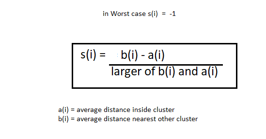
Inertia is not a good performance metric when we try to choose the value of ‘k’ since it keeps getting lower as we increase the value of ‘k’. A technique that is best used to find the number of ‘k’ clusters is to use the silhouette coefficient. The silhouette coefficient is given by

The silhouette coefficient can vary between -1 and 1. A value of 1 means the instance is very well in its own cluster and far from the other clusters. A coefficient value of 0 means the instance is located close to the boundary. A value of -1 means that it has been assigned to the wrong cluster. In sklearn to find the silhouette scores you can always use silhouette_score(). Silhouette diagrams are a visual representation of this and are always useful.

Limits of K-means

Despite the fact that this algorithm is fast and scalable, this method is far from accurate as the due to the fact that this has to be run multiple times and the process to find the value of ‘k’ is also quite tedious. At the same time K-means do not tend to behave properly if the clusters are of varying sizes.

---

Clustering can be used as an efficient approach to dimensionality reduction, in particular as a pre-processing step before a supervised algorithm

---

DBSCAN

This algorithm defines clusters as continuous regions of density. The algorithm is as follows:

1. Find the points in the ε (eps) neighborhood of every point, and identify the core points with more than minPts neighbors.
2. Find the connected components “Connected component (graph theory)”) of core points on the neighbor graph, ignoring all non-core points.
3. Assign each non-core point to a nearby cluster if the cluster is an ε (eps) neighbor, otherwise assign it to noise.

DBSCAN does not have a predictmethod but only a fit_predict method

Other Clustering Algorithms

Agglomerative Clustering

A hierarchy of clusters is built from bottom up. At each iteration, this algorithm connects the nearest pair of clusters

Birch

Built for large datasets and faster than K-means as long as the features are less than 20

Mean Shift

Algorithm starts by placing a circle centered on each instance. For each circle it computes the mean of all instances located in it and then shifts the circle so it is centered around the mean. It keeps iterating until the circle no longer moves. The algorithm shifts circles into a direction of high density. Finally all instances whose circle have settled is the place that forms a cluster. This is not suited for large datasets and it tends to cheap clusters into pieces if they have internal density variations

Spectral Clustering

Algorithm take a similarity matrix between instances creates a low dimensional embedding from it. If then uses another clustering algorithm in this low dimensional space